This article is a summary of Chapter 1, section 4-6 of:

Arpaci-Dusseau, R. H., & Arpaci-Dusseau, A. C. (2023). Operating Systems: Three Easy Pieces (1.10th ed.). Arpaci-Dusseau Books.

The scheduling algorithm is used to manage the CPU resources among multiple competing processes, in order to make sure each process receives fair amount of CPU time to complete its task. Metrics for evaluating scheduling algorithms include turnaround time, the time it takes for a job to complete when it enters the system, and fairness (such as Jain's fairness index), whether the CPU time is divided fairly among all jobs. In the rest of the article, I will introdue a few basic scheduling algorithms.

Common Scheduling Algorithms

First-in-First-Out is probably the easiest implementation of a schedular, which each process is executed in the order of arrival, and a process gets executed only when all the processes before it complete. However, this approach has a serious limitation knwon as convoy effect: when a few short processes are queued behind a heavyweight process, they must wait for the heavy process to complete. For example, assume that process A takes 100 seconds, and B, C only take 10 seconds.The turnaround time of the schedular is (100 + 110 + 120) / 3 = 110s.

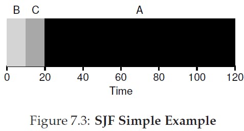
Shortest Job First (SJF) solves the problems by always queuring the jobs in the order of increasing running time. Thus, the shorter jobs always run before longer jobs. In theory, this approach can achieve the minimum turnaround time. Back to our previous example, the turnaround time of SJF is (10 + 20 + 120) / 3 = 50s, less than half of first-in-first-out.

However, SJF only works if the shorter processes arrive earlier or at the same time as the longer processes. Assume that A arrives earlier before B and C and is scheduled by the OS, we are then back to the first senario where B and C are scheduled behind A.

A solution to this problem is to utilize the preemptive multitasking generally supported by modern operating systems, that is, instead of letting the process run until it completes, the operating system regains the control of CPU during every timer interrupt and is able to switch to another process. Preemptive Shortest Job First (PSJF, also called Shortest Time-to-Completion First STCF) compares the running time of a new process with the current process when a new process arrives, and switches to the process that has shorter running time.

As computer becomes more interactive, a new requirement, response time, emerges in addition to turnaround time. Since users would not want long latency of interactive programs, processes that interact with users should not be waited for a long time to be scheduled. Response time is measured as the time between the process being first scheduled and the time of its arrival.

Round-Robin (time-slicing) is an algorithm that optimizes response time. Instead of waiting for a process to complete, it runs each job for a given amount of time slice and switches to another process. Thus, each process has the same opportunity to interact with the user in short latency. Since context switch can only happens at timer interrupt, the time slice must be a multiple of timer-interrupt period. Determining an appropriate time slice is crucial such a slice that is too long leads to longer response time, and too short reduces the effiency of the operating system by frequent context switch.

A trade-off of Round-Robin is that it has the worst turnaround time, since it is essential entending the total running time of each process for as long as possible.

Multiple Layer Feedback Queue

The shcedular algorithms we described above are all theoretical models, since they all assume the running time of each process is known. However, in reality, there is no way for the operating system to know how long it takes a user process to run. The idea behind a Multiple Layer Feedback Queue algorithm is to predict the future running time of a process based on its current behavior.

Multiple Layer Feedback Queue (MLFQ) stores processes in a number of queues with different priority level. It always runs the processes in the higher-priority queues before scheduling processes in lower-priority queues. If there are multiple processes with the same priority, they are scheduled with Round-Robin algorithm. Importantly, the priorities of processes will be changing in time based on their observed behaviors.

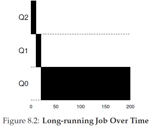
A simple model of the priority changing algorithm is as follows: when a process enters the system, it stays at the queue with highest priority. If the process uses up an entire CPU time slice, it is likely to be a CPU intensive process that has lesser requirement on response time. Thus, its priority level is reduced. If a process gives up the CPU before the end of time slice, it is probably an I/O intensive interactive program, and it maintains the same priority. This algorithm tends to approximate STCF algorithm, where shorter jobs are assigned before longer ones, as shown in Figure 8.3.

However, there are three problems with our simple approach:

1. If there are too many high-priority interactive processes, the long-running processes may starve.

2. A long-running process may changes its behavior to an interactive one while still remaining in the lower-priority queue.

3. A user program can trick the scheduler to maintain it at high priority by issueing periodic I/O calls to give up CPU.

To solve problem 1 and 2, we uses a method called priority boost: moving all processes to the highest-priority queue after a given time interval S. This allows even low-priority tasks to have some share of CPU time and not being starved. It also enables a long-running process that changes to an interactive one to regain high priority if it stays interactive. In practice, an appropriate value of S need to be fine-tuned through experiments. A value that is too long wil not provide lower-priority processes with enough CPU resource, while a value that is too short will disrupt the functioning of scheduling algorithm.

To solve problem 3, we can modify the rule of switching priority. Instead of determining whether one process uses up the CPU time, each process can only maintain at a priority level for a given time slice. Usually the higher the priority, the shorter the time slice allowed. When the time slice for one priority level is used up, the process moves to the next level. In this way, since we are not considering how the process uses up the time slice, the user program cannot trick the scheduler. Combining this method with priority boost, we can still maintain the behavior of MLFQ: the shorter-running processes that uses time slices slower remains on higher priority, while longer-running processes that uses time slices continuously move to lower priority quicker.

In summary, here is our modified rules for MLFQ scheduling: